A Guide To Creating Your Own Homeless Encampments Dataset

In an effort to increase the research, understanding, and support of homeless communities outside of Salt Lake City the following guide was created. This guide walks through the design, implementation, and maintenance of a geographic database similar to the SLCHED. Built on open-source platforms, the tools needed to recreate a homeless encampments dataset for any location are available to everyone. With some time and effort anyone can recreate this project, helping to better understand the factors that influence the movement and placement of encampments within their own city. All the required SQL code for this project can be found HERE in a copiable text document. While the SLCHED is not an open dataset, due to the risks associated with exposing the location of current camps, we hope that others can learn from this guide and begin to critically engage with the homeless geographies that surround them. If you are interested in the SLCHED specifically for research or activism, please contact us via email.

The Database

The SLCHED is implemented through a PostGIS database. This object-relational database structure was chosen at it allows for quick and efficient queries of the data through structured query language (SQL) coding. PostGIS is a spatial extension to PostgreSQL. Developed for over two decades, PostgreSQL stores data in relations (imagine spreadsheet tables) which allow it to be efficiently indexed and queried. PostgreSQL databases also meet the ACID standard of atomicity, consistency, isolation and durability allowing them to be simultaneously updated by multiple users with no fear of loosing or overwriting critical data. The PostGIS extension of PostgreSQL provides additional relational objects such as geometry and geography that allow for the indexing and quiring of spatial objects (lines, polygons, multipoints, etc.…) within coordinate or projected space. Utilizing a PostGIS framework the SLCHED is able to map individual encampments through space and time while simultaneously recording non-spatial information such as times of documentation, dates of collection, and weather information. The flexibility of these databases is matched by their small storage size, as features are stored as lines of well-known-text (WKT) within relations. The entire SLCHED, documented for a year and half, can be backed up into a single plain text file that is under 750kb.

Software installation

To create your own homeless dataset three pieces of software are required, PostgresSQL, pgAdmin 4 and QGIS. PostgreSQL is the underlying database software required to create relations and store data, pgAdmin 4 is a user-friendly backend package which manages the database and makes for easy backups, while QGIS is used for visualization and to update camp polygons as needed. The initial installation and setup of these software packages can be intimidating and time intensive, but once appropriately set up they are easy to utilize and maintain.

PostgreSQL, along with the PostGIS spatial extension and pgAdmin 4 management tools can all be downloaded here. Simply download the newest version for your operating system and run the graphical installer wizard. Detailed instructions for the graphical installer can be found here. Make sure that you select all four components (PostgreSQL Server, pgAdmin 4, Stack Builder, and Command Line Tools) to be installed. You will also be prompted to create a superuser password for the default username postgres. This will be required to access your database through pgAdmin 4 or QGIS. If you forget it, you will lose all access to your data. You will be required to enter your username (postgres) and your password frequently so make sure it is memorable. Once the setup wizard for PostgreSQL is completed it will prompt you to launch the Stack Builder, make sure you do so. Stack Builder will create a PostgreSQL server along with the additional spatial components required for this work. In our case you need the basic PostgreSQL and to select the most current PostGIS build under the spatial extensions options. Once selected you can proceed through the wizard to complete your download and installation. As mentioned earlier the initialization of PostGIS can be quite involved. We would recommend reviewing these resources for additional guidance, An Almost Idiot’s Guide Installing PostGIS on Windows and How to use pgAdmin.

Thankfully QGIS is a more straightforward installation process. Simply download the long-term release appropriate for your device from this page and follow the installation instructions. While you can opt to download and install the latest release, which typically has more features, the stable releases are still feature rich and ensure that QGIS will easily connect with pgAdmin 4 with little to no headaches.

Database Structure

To ensure the optimal functioning of your homeless database you will need to provide it with a structure conducive to the data being collected. Relational databases use a system of Primary and Foreign Keys to allow for the storage and quiring of data. A Primary Key within any relation is a unique entity (never repeated) that links rows of information on the given object. Foreign Keys are data within a relation that are not unique (may be repeated) but are primary keys for another relation within your database. How these keys are utilized and connected to form a consistent database structure will be detailed following the entity-relationship (ER) model visualized below.

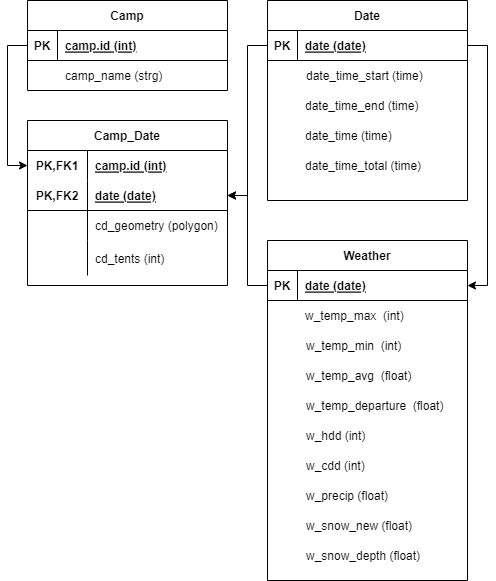
Within this framework two primary keys are used, camp_id and date given as integer and date formats respectively. The camp_id is held within the Camp relation. The Camp relation lists the documented camps, as camp_id integers and links them to their camp_name given as a string. This allows you to keep track of how many individual camps you have found, while linking them to more easily remembered names.

The date primary key is used within both the Weather and Date relation. This shared key makes it easy to link or join these tables giving you weather data associated with a specific date of documentation. The Weather relation links dates (every calendar day) to specific meteorological conditions recorded for the given day. In the case of the SLCHED these include max and min temperatures, average temperature, and precipitation data.

Within the Date relation only days of camp documentation are recorded. Along with the date the start and end times of recording are also noted along with the average recording time and total time spent documenting.

Our final, and most critical, relation is the Camp_Date relation. This relation stores the geometry, spatial polygons, and tent counts for each recorded encampment. This is accomplished by using the foreign keys, camp_id and date, to create a unique compound primary key, poly_id. In effect this means that each encampment, referenced as a poly_id, is actually defined by its camp_id and date of recording. This allows us to query our database for all encampments of a given camp_id and count the number of days they were canvased and the given weather and recording conditions for that day. Or we can query a specific date and note which camp_ids were associated with it. This structure allows us to monitor individual encampments as they grow and shrink through time, while also detailing the total number of tents recorded for a given day and how this might be fluctuating with weather patterns.

Database Implementation

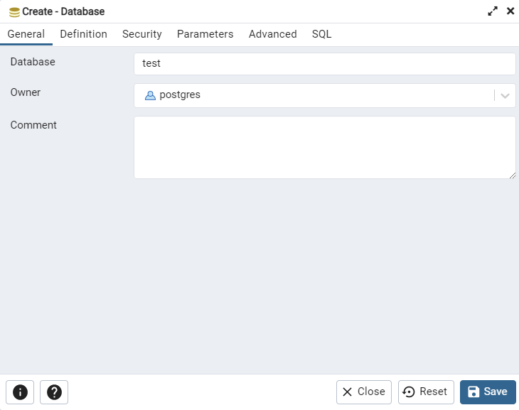
To implement this database structure first open pgAdmin 4. It will prompt you to provide your password. Once at the home page you can select servers, and right click on PostgreSQL 13 to create a new database. In this example we are calling the database test, but you should name your database more appropriately. Simply click save, no need to change the default settings, and a new database will appear.

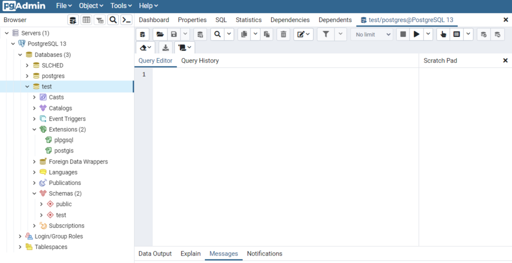
However, keep in mind this is only a PostgreSQL database with no ability to manage geographic data. To do this we will enable the PostGIS extension we previously installed using Stack Builder. To do this right click on your database and select Query Tool, which will give you this view.

The Query Tool allows you to run SQL commands on your database. We will be entering the several commands which we will run by pressing the play button in the upper right of the window.

All code demonstrated in this guide is provided here, and at the end of the guide. You can copy and paste from this text file to make your life easier, just remember to change any reference to slched to the name of your new database.

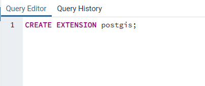
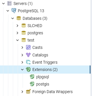
This code, as you might have guessed, activates our PostGIS extension. If you refresh your database and examine your extensions, you will now see PostGIS appear alongside the standard plpgsql extension. More detailed instructions on enabling PostGIS, and its other features, can be found here. With our database established we can close pgAdmin 4.

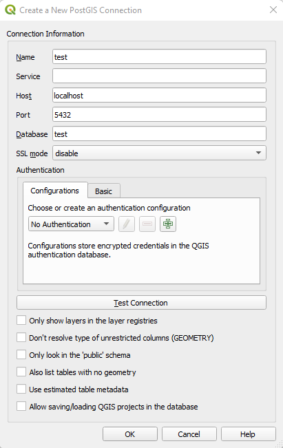
Open a new project in QGIS. In the top menu select Database and DB Manager. Right click on PostGIS and select New Connection. This will create another window requesting information related to your database. Name is what you want to refer to your database as within QGIS, Host should be set to localhost, leave Port as 5432, set Database to the name of your database within pgAdmin 4, leave all other options default and click OK.

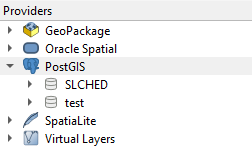
You will now be prompted for your pgAdmin 4 credentials (remember your username is postgres). Clicking on the PostGIS option should now show your database. You can now save this project using the blue floppy disk icon. Congratulations you have successfully deployed a PostGIS database that is linked to a QGIS project!

Database Creation

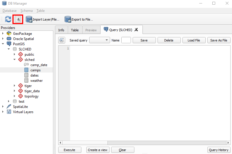
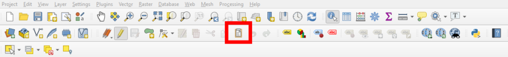
With our database implemented we can begin to structure it as described by our entity-relationship model. To do this select your database within the DB Manager and click the SQL Window button (it appears as a wrench on top of a word document). Like the query tool in pgAdmin 4, this window will allow you to run SQL code to create, update, and query your database.

To begin we will create a schema to hold our relations. Schemas can be thought of as folders which hold specific relations that are typically queried together. The SQL code to create schemas is given below

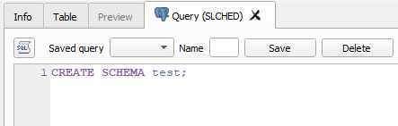
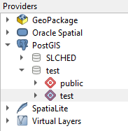
You can name your schema whatever you like, in this case we are going to call it the same as our database. Once run you can refresh your database, the refresh button is in the upper left of the DB Manager window, and you should see a new empty schema called test.

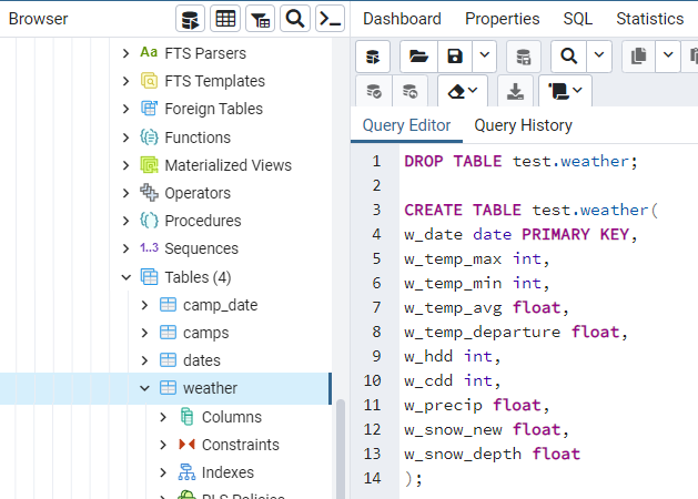
Navigating back to the query tool we can enter the following lines of code to create our empty relations. First the camp_date relation.

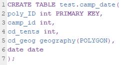
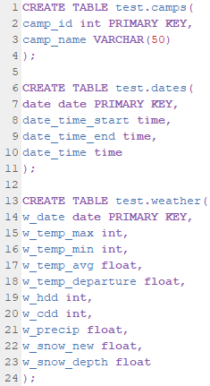
Line 1 creates a new table called test.camp_date. This phrasing gives the name of the schema, in our case test, followed by the relation itself. We can then see that each field is created with lines 2 through 6. Note that the types of data allowed in each field are defined, int for integers, date for dates, and geography in the form of polygons for our camp outlines. Also note that poly_id is defined as the primary key. We will repeat this process for our other three relations (camps, dates, weather). In each code chunk you can see the various inputs and their allowed datatypes along with the relation’s primary key. Copy and paste this code from the code document found at the end of this guide, making sure to update this code to replace “test” with the name of the schema you created earlier.

The Data

Now that we have a database implemented and its relations set, we need to fill it. There are three steps to data processing for the SLCHED. The first is canvassing, in which we search the city for encampments and record their locations. Canvases are followed by camp documentation in which we create the polygons within our database representing these recordings. Once the geographic location of camps is determined we can collate weather information and upload it to our database. Each of these methods will be covered in detail below.

Canvassing

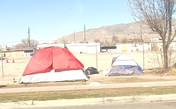
Canvasing for the SLCHED is conducted via car, with camps documented using video footage. On average, a city-wide canvas takes about one to two hours to complete. During a canvas, all known active camp sites are visited, as well as any sites of previous encampments. Returning to previous camp sites allows for the documentation of potential re-growth that occurs after abatements. New camps are found through communication with the homeless and local activists, by reviewing the map of Salt Lake City cleanup calls, and serendipitously on regular canvasing trips. Potential encampment locations are canvased alongside active and past camp sites.

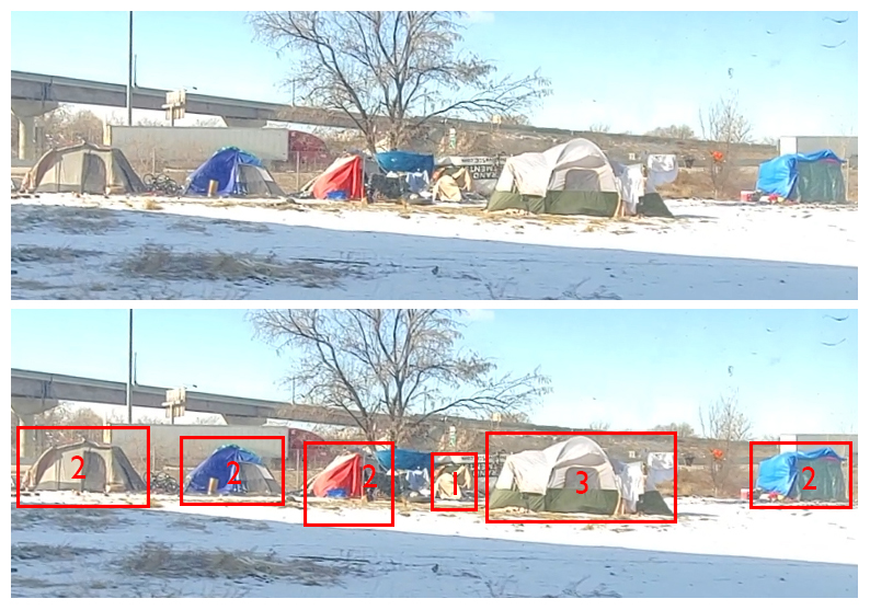
Within the dataset, an encampment is defined as tents or covered structures (i.e. tarps over a canopy or between railings) capable of housing two or more people. Tents vary in size from single occupancy structures to larger shelters capable of holding multiple people. For the SLCHED a single occupancy tent alone is not considered an encampment but is worthy of further documentation in case of growth. A larger tent that could hold two individuals, or two single occupancy tents, is documented as an encampment in its own right. As encampments grow any structures within approximately 10 meters of each other will be identified as a single encampment. Campers within encampment tents would be considered likely to interact on a daily basis forming a single unit. For tent counts within an encampment, single occupancy tents or similarly sized structures are considered a single tent. Larger structures, such as two, three and five person tents are counted as multiple tents based on how many individual tents could fit within them. In many cases multiple single or double tents will be linked together with a tarp or covering, and it is common to see shelters built in various ways utilizing discarded materials available to the homeless. These built structures are challenging to count consistently and require canvasser interpretation. However, as canvasing continues you will develop a feel for how many “tents” should be counted for larger built structures. Over the year that Salt Lake City has been canvased the two primary documenters have become attuned to these values, frequently suggesting the same tent counts for even the most challenging encampments composed of multiple built structures.

When utilizing this canvassing method there are several limitations to your dataset that should be kept in mind. First is that it will take you time to find all of the regular encampment sites within your city. As you canvas more frequently you will get a feel for where camps are located, and your average tent and encampment counts per canvas will increase. Expect that at least your first month of documentation will underestimate the true size of your homeless population. Also keep in mind that tent documentation does not equate one-to-one with homeless population size. There have been instances where a single tent has housed many homeless individuals while in other cases a single individual might use multiple structures to protect themselves and their belongings. We have often found it challenging to capture new encampments the day they arise, often finding or hearing of them a few days later. This makes your dataset more valuable as a tool to track the growth and change of camps than as a strict survey of every encampment in your city. Also be aware that this method only documents camps visible from a car, while we know of camps (sometimes quite large) that are located along rivers or mountain trails. Unfortunately given the time constraints of canvasing these camps remain undocumented. If the time and resources are available, we would encourage you to supplement your canvases with data collected by walking around potential campsites on foot. It is also best practice to have more than one canvasser. The SLCHED was initially documented by a single researcher which led to missed days and inconsistent documentation due to scheduling overlaps or sickness. Having at least two canvassers can mitigate these issues while also decreasing the burnout that constant canvasing can produce.

Camp Documentation

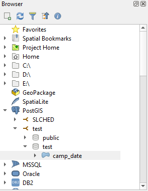
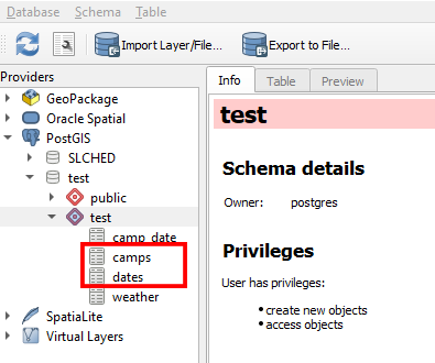
During camp documentation video footage of each canvas is reviewed and translated into polygons and tent counts within the database using QGIS. To accomplish this, you will need to open the QGIS project you previously linked to your database. You do not need to run pgAdmin 4 at the same time, but you will be asked to sign in. First select an appropriate base map to reference when creating your polygons. Here is a useful resource for downloading additional base maps into QGIS, https://opengislab.com/blog/2018/4/15/add-basemaps-in-qgis-30. Now you must add your database as an editable feature layer to your project. To do this select your database using the browser on the left-hand side of the screen. Clicking PostGIS you should see your database and available schemas, under your schema there will be a single option camp_date, as this is the only geographic relation in the database. Right clicking on camp_date you can select Add Layer To Project.

It is recommended to right click camp_date under layers and check the Show Feature Count Box, this will inform you how many unique camp polygons are in this relation.

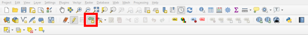
The geographic extent of each camp is defined by the furthest outlying tents. Polygons are traced around these tent outliers, which determine the camp boundaries. Any spaces between tents are included within an encampment polygon. To add an encampment polygon select the yellow pencil button which toggles layer editing on and off.

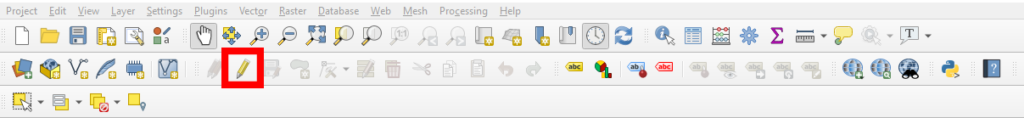
This will allow you to select the Add Polygon Feature button, which appears as a green blob with a yellow star.

Using the cross hair, you can left click to add vertices to your encampment polygon. Right clicking will finish your selection and create the polygon. This will open up a Feature Attributes window in which you can add information to the given spatial feature.

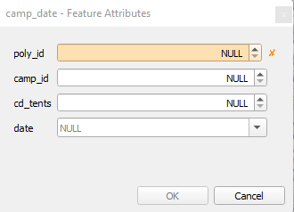
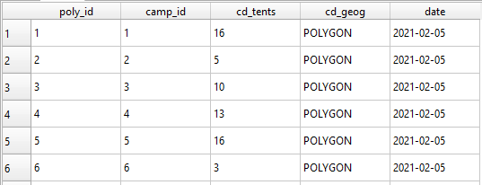
The poly_id, highlighted in orange, is the Primary Key and is required to add a polygon feature. Looking at your feature count for your camp_date layer will let you know the current number of polygons that you have created. Your new feature should have a poly_id that is one larger than this number. While you can input any number into this field keeping it consistently incrementing upwards helps to maintain a consistent database. You must then enter the camp_id associated with this encampment. If you are creating a new polygon for a camp which already exists, or has existed in the past, make sure to keep this value consistent. The next field, cd_tents, is a count of how many tents/structures reside within the given encampment and date is simply the date of canvassing.

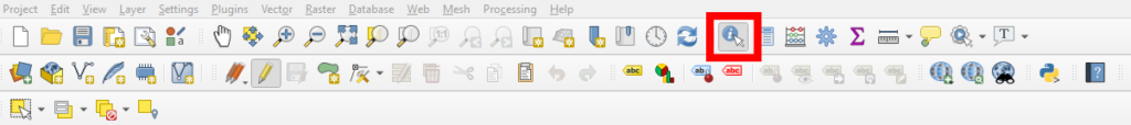
After establishing regular encampments, it is typically easier to copy and paste features, as opposed to redrawing every encampment for every canvas. This is particularly true if the spatial extent of the camp has not changed. To do this you can select the previously documented polygon with the Select Features tool, which appears as the letter “i” with a mouse curser over it.

Using this tool will select every polygon over time that has existed within this space. Each polygon will appear on the right side of the screen under Identify Results.

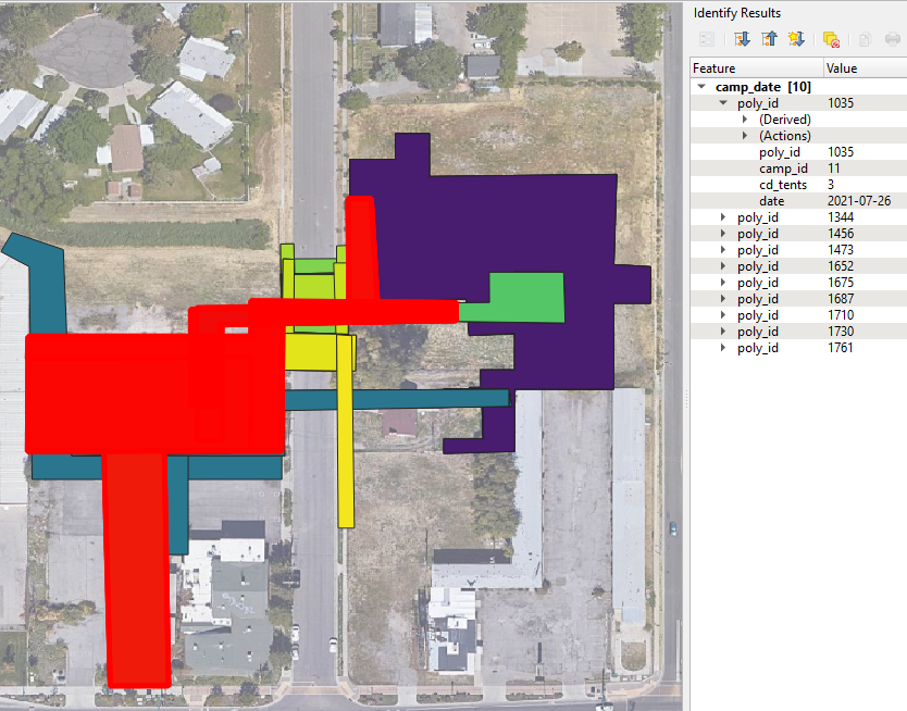
Using this menu, you can right click on the poly_id you are interested in copying and select Copy Feature. To place a copy of this polygon into your layer simply click the Paste Features button, which appears as a clip board icon in the tool bar. This will open up a new Feature Attributes window which you can fill with the appropriate data for that particular canvas date.

Once you have created polygons for every encampment recorded on the given canvas make sure to toggle off editing using the yellow pencil. This ensures you do not accidentally add additional polygons. And of course make sure to save your progress frequently using the blue floppy disk icon.

As more dates of canvasing are added it will become challenging to add additional polygons given the visual clutter of persistent camps. To assist with this, you will want to enable the Temporal Controller for you camp_date feature layer. This can be done by double clicking on the layer opening the Layer Properties window. This window allows you to adjust the symbology of your polygons and other attributers of the feature. What you want is the Temporal options, identified by the clock icon.

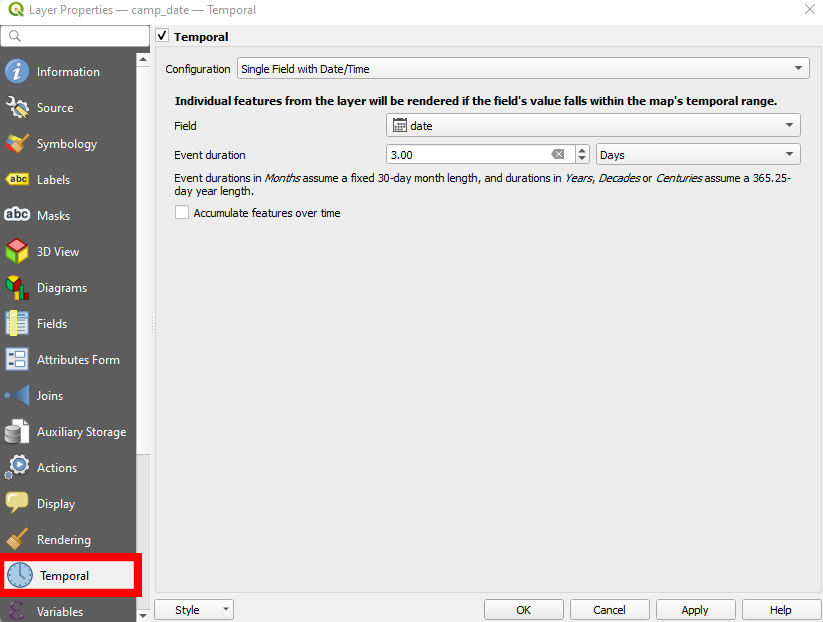
On this page set the configuration to Single Field with Date/Time. This will allow you to set the field as date and determine an event duration. In the image above this is set to every 3 days, the temporal resolution of the SLCHED, you should set this to match the temporal resolution of your database. Make sure to click Apply and then OK in the bottom right after making these adjustments. You will now have a Temporal Controller appear above your project map.

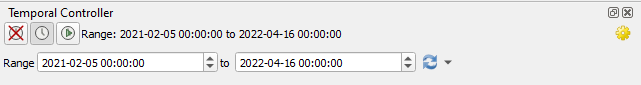
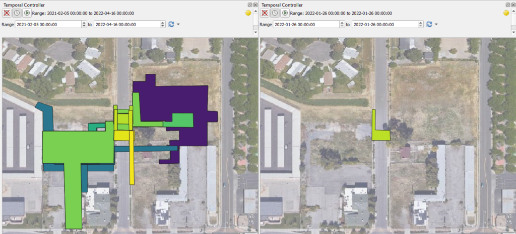
You can adjust this to display encampment polygons over specific time periods. From the entire duration of your database to a singular date. This controller can help you find specific polygons to copy and paste, reference spatial areas to see if camps have historically existed there, and generally make your time documenting camps through QGIS more efficient and tolerable.

With your encampment polygons in place, you can now update the dates and camps relations using QGIS. To do this navigate to the DB Manager window under Database. You can find these relations under your schema located below your database and the PostGIS tab.

Right clicking on each relation will give you the option to Add to Canvas. This will place them within your layers in the bottom left of the project, beneath your camp_date feature. While these relations do not have spatial extents, they can be edited by right clicking on them and selecting Open Attribute Table. This will open a window displaying the relation as a table. In the upper left you can again toggle on editing using the yellow pencil icon. This will allow you to create new rows of data using the add feature button, represented as a yellow row being added to a table.

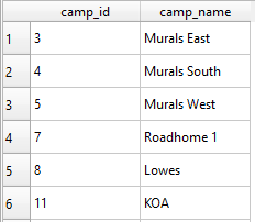
This button will create a new row within the table that needs to be filled. For the camps table simply add the camp_id that you have used for a given polygon and then assign it a name. It is recommended to use cross streets for these names or well-established landmarks. Sometimes multiple camps will form close to a given landmark. In these cases, it is recommended to differentiate them using numbers associated with which camp was documented first. In the case of the SLCHED there is a Foss 1 and Foss 2 camp, both of which are located along a road with no cross streets to reference.

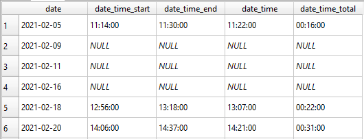
For the dates relation you will need to include the date that the canvasing took place. All the other fields are optional, however including data within them will allow for more detailed analyses. The date_time_start column is the time that the canvasing started. For the SLCHED this is the time stamp of the first video recording of a camp. Similarly, the date_time_end designates when the canvassing ceased, and for the SLCHED is marked as the time stamp of the last video recording. The date_time column represents the general time of recording. This is given as the mid-point of a specific canvas. Having this value allows us to determine when camps are being recorded and to find temporal patterns in camps sizes, potentially mitigating these biases by recording during a consistent time of day. The final column, date_time_total, is the amount of time in hours that the canvas took. This allows us to review if longer canvasing times are biasing our tent counts towards larger numbers. Again, make sure to toggle off editing after each entry creation and to save your progress frequently.

Weater Data

While not required for spatial analysis, having access to weather data within your database will allow you to examine encampment trends related to material conditions outside of police and health department pressure. For the SLCHED weather reports are collected from the National Oceanic and Atmospheric Administration’s NOWData portal, https://www.weather.gov/wrh/climate?wfo=slc. The methods outlined below should be adapted to the closest weather monitoring station to your geographic area.

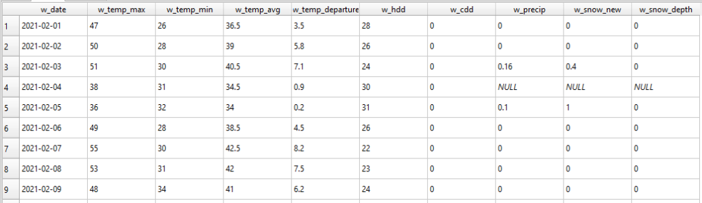
Weather data is added to the database on a monthly basis. The weather relation holds information regarding max, min, and average temperatures along with temperature departures and precipitation data. The columns used match up with those provided by the NOWData portal. However, you are free to remove columns which you find non-useful. To collect data, select the Daily Data for a Month weather product for your given location and time frame. This will produce a chart like this

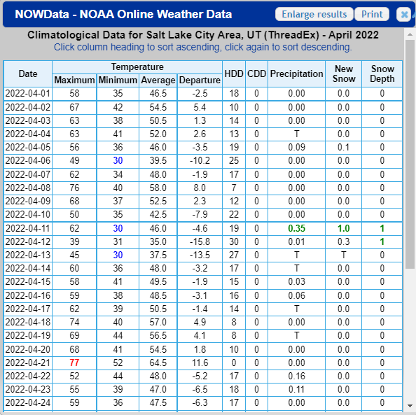
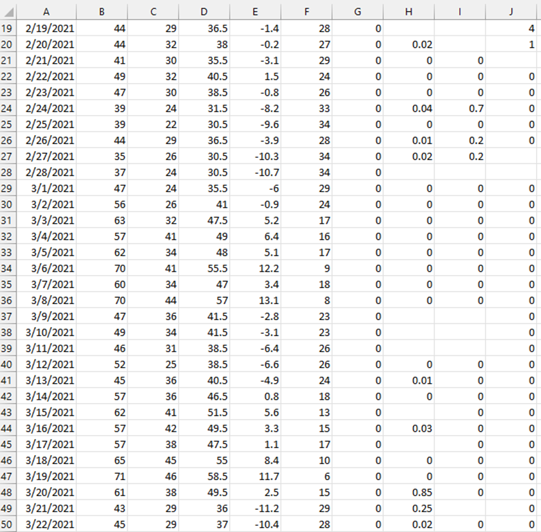
These cells can then be copied and pasted into an Excel sheet, or similar spreadsheet data management tool like Google Sheets or LibreOffice Calc. Make sure to copy over all the data for each day of the month, avoiding the Sum, Average, and Normal rows found at the bottom of the data product. You will find that in some of the precipitation entries a letter, often T or M, is used in place of numeric values. These will need to be deleted from your spreadsheet. Save this spreadsheet as a .CSV file.

As your encampment canvassing progresses you will copy and paste additional weather data into this saved .CSV file. Below you can see the entries for the SLCHED spanning two months, with non-numeric values deleted.

You will add this weather information to your database using pgAdmin 4. To do so open the pgAdmin 4 application on your computer. It will require your password at launch. Using the left most panel navigate to your weather table within your database. This will be located under PostgreSQL 13, Databases, your database, Schemas, your schema, and Tables. Right clicking on weather will give you the option to Import/Export Data… Selecting this produces the given window.

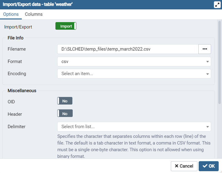
Make sure to update the Import/Export option to import. Then select your .CSV file from your computer and use csv as the format. You will not need to select an Encoding option. Click okay and your weather data will be added to your database.

After your initial import you will need to update this weather table every month in order to do up to date analyses. Updating your weather data is a bit more involved. To do so you will have to delete/drop your previous weather table and then recreate the table and import your new extended weather dataset. To do this right click on your weather table and open the Query Tool. From here you can use the following code to drop and recreate your table.

Once recreated you can simply follow the same import procedure to fill your empty weather table with up to date information.

Back Ups

As mentioned earlier one of the benefits of using a PostGIS database is the minimal storage necessary to save and back up your data. It is encouraged that you back up your database after every documentation. Trust us, redrawing encampment polygons is not a fun time.

Backups are made using pgAdmin 4. After signing in navigate to your database under PostgresSQL 13 and Databases. Right clicking on it will give you the option to Backup…, which opens the following window.

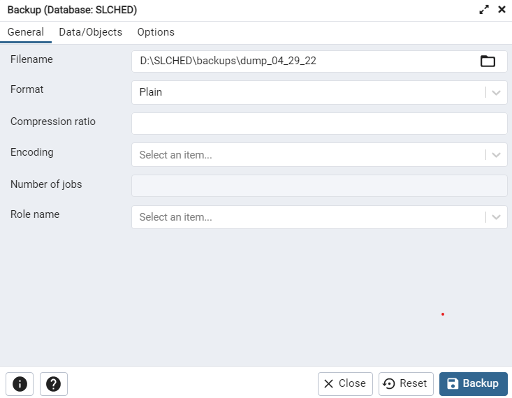
Filename will determine where your backup is saved on your computer. For Format select Plain leaving all other options blank and click Backup. This will create a plain text backup of your database. This document steps through a series of SQL commands that will recreate your database structure and refill your database relations, should something happen to your local files. We would recommend saving these regular backups off site to ensure you do not lose your data, should something happen to your local machine.

To utilize these backup you will need to create a new server and database using the PostgreSQL graphical installer and Stack Builder. Once your basic database is established open pgAdmin 4 and navigate to the PSQL Tool under Tools. The PSQL tool has many lines of dialogue at the top when you open it. You will enter code at the section near the bottom that shows the name of your database followed by =#.

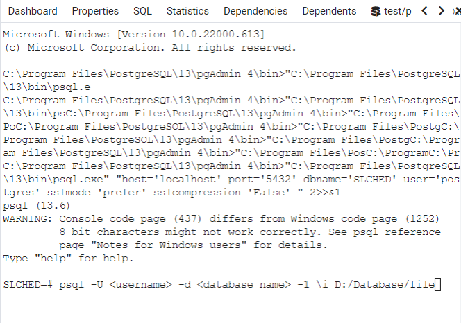
Enter the following line of code, replacing <username> with postgres, <database name> with the name of your backed up database, and D:/Database/file with the location of your plain text back up on your local machine. This will run the plain text backup restoring your database structure and all previously entered data. Relinking this to a QGIS project will allow you to continue your work where you left off.